Games Series #1 Simulating a Rope
Prerequisites. To understand the techniques presented in this article, the reader is recommended to have a basic understanding of calculus, linear algebra, and classical mechanics. Specifically, the reader needs to be familiar with the concept of integration, differentiation, differential equation, position, velocity, acceleration, and force. Familiarity with basic game development patterns such as the game loop and the idea of a physics engine will be of great help when putting everything together.
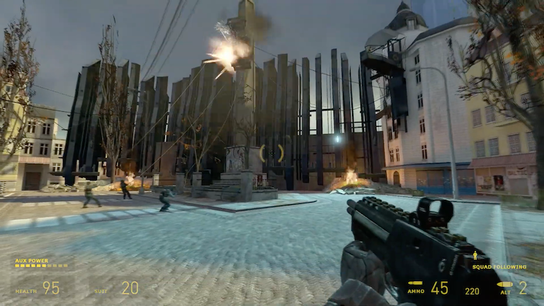
Half-Life 2 was a pivotal point in the industry of video games. I played through it many times, admiring its beautiful graphics, its challenging puzzles, and, of course, its top-notch storytelling.
Although not the first to integrate the Havok physics engine, the second instalment of Half-Life differentiated itself by making it a first-class citizen. Physics was showcased in a way that served the narrative. There is one scene in particular that I remember—in the chapter “Anticitizen One,” members of the resistance group bring down a propaganda billboard screen by pulling it down with ropes. It was symbolic, and an excellent use of ropes in level design and interactive storytelling. Throughout Half-Life 2, ropes are not just static objects; they appropriately respond to and affect the world around them.
In this article I present a method for simulating such ropes in videogames. I shall use simple two dimensional examples, but the idea can easily be extended to support three dimensional worlds. In fact, it’s the same technique used by Unreal Engine 5 in the implementation of their cable component.
1.1 Ropes in Real Life
I believe that in order to better use an object in a video game, one needs to have some general knowledge about it in the real world. This helps with design decisions—where, when, how do we use this in the game? What mechanics can it enable? Understanding the real world properties of the object and of the materials that the object may be made of might also influence various implementation decisions—how should this object look? How should it interact with other objects in the game?
Consequently, I believe a bit of background about ropes is in order. To make a rope, we start with some fibers. Those may be natural (hemp, linen, cotton, etc) or syntehtic (nylon, polypropylene, etc). We twist those fibers together into what we call yarns, and those yarns into strands. Finally, we twist those together to make rope.
The origin of rope dates back to prehistoric times, and through the years it played an important role in the development of humankind. Rope can be made by hand, but since about 4000 BC, people started using machines to make it. It is believed that the Egyptians were the first to invent such devices, probably because rope was indispensable to their agriculture and the building of their structures, including their temples and pyramids. They usually made rope out of materials such as water reed, date palms, flax, grass, papyrus, leather, or even camel hair.
One well-known method of making rope employs the concept of a ropewalk—a technique used mostly by Europeans in the 17th and 18th centuries. You can see how it works in Science Channel’s short video from below, from their How It’s Made series.
If you're interested in more, you may watch Ropewalk: A Cordage Engineer’s Journey Through History (available for free on YouTube), a documentary in which Bill Hagenbuch talks about the history of rope making in the United States at the Hooven & Allison company. Even more resources are available at storyofrope.org.
1.2 Ropes in Video Games
In video games, we do not need to simulate the real world with perfect accuracy, instead we are interested in techniques that give us most fidelity at a low computational cost. In the case of rope, we do not simulate the individual fibers, yarns, or strands. Instead we model ropes as systems of particles constrained to sit together in a shape that, to some extent, resembles the real thing. More like a chain than a rope. It is only during the rendering process that we visually connect those particles to make them look like a rope. We would like to retain the physical properties and the way they act on the world, meaning we may want to use our virtual ropes for dragging, pulling, lifting, or suspending other game objects. We may also want them to break if enough force is applied, or the ability to cut them at will, such as in the 2010 hit game Cut the Rope.
1.2.1 The Equations of Motion
You should already be familiar with the idea of rate of change. That is, if an object has position \( s(t) \) at time t, then the rate of change of its position is called velocity, and is given by \( v(t) \) = \( s'(t). \) The rate of change of the velocity is called acceleration, and is given by \( a(t) \) = \( v'(t) \) = \( s''(t). \)
In game physics, we are interested in calculating some future position of an object based on its current position and the forces acting on it. Newton’s second law of motion says that the net force acting on an object is equal to its mass times its acceleration, \( F(t)=m \, a(t). \) By dividing by m, we obtain a way to compute the acceleration of an object at a given time: \[ a(t) = \frac{F(t)}{m}. \] Since we are interested in computing the position of the object, we need to use this information in reverse: \[ \begin{align} v(t) &= \int a(t) \, dt, \\ s(t) &= \int v(t) \, dt. \end{align} \]
1.2.2 The Case of Constant Acceleration
If we know the acceleration to be constant, we can get away with a beautiful analytic solution. Say \( a(t) = a_0, \) a constant, then we may solve for the velocity, \( v(t), \) as such—\[ v(t) = \int a_0 \, dt = v_0 + a_0 t, \] where \( v_0 \) is \( v(0), \) the velocity at time \( t=0. \) Furthermore, given the velocity, we can get the position, \( s(t) \)—\[ \begin{align} s(t) = \int v(t) \, dt &= \int (v_0 + a_0 t) \, dt \\ &= s_0 + v_0 t + \frac{a_0 \, t^2}{2}. \end{align} \] This is fairly easy to implement, and results in a bare bones physical environment. In the interactive example below, we have only one type of object—a ball, and only one force acting on it—gravity, which pulls the object downwards. Press anywhere on the canvas to create a ball. Press and drag to choose \( v_0. \)
This is what we call an analytic approach. The position of each ball you throw is determined solely by a function of time. The advantage of this approach is that it’s completely accurate. Its disadvantage is that it’s not very versatile. Actually, it’s usually not even possible to find an analytic solution. Physical systems are described by differential equations, but those equations are most often not solvable analytically. Take the example of a simple pendulum. A pendulum consists of a body of mass m, suspended by a massless string of length L. As the pendulum swings from one side to the other, we want to compute the angle at which it is situated at a given point in time. The differential equation that describes this kind of system is \[ \theta''(t) + \frac{g}{L} \sin \theta(t) = 0, \] where g is the acceleration due to gravity and L is the length of the pendulum. This system is not solvable analytically! It does becomes solvable when it is assumed that \( \theta \) is so small that the difference between \(\sin \theta\) and \( \theta \) is negligible. Only then do we get the well-known analytic solution, also known as simple harmonic motion: \[ \theta(t) = \theta_0 \cos \left( t \sqrt{\frac{g}{L}} \right). \] Since most equations can’t be solved analytically, we need a way to simulate what’s happening without knowing the underlying master functions. We need to introduce the concept of numerical integrators.
1.2.3 The Euler Method
A numerical integrator is an algorithm that calculates integrals numerically. There is an entire subfield of mathematics that studies numerical algorithms, called numerical analysis. These algorithms, as opposed to analytic formulas, are not completely accurate, so there is some kind of error involved. However, in video games the physics needs to look good and not take long to compute. As long as the result is believable, the physics does not need to be very accurate. With this being said, accurate methods tend to produce desirable results, so we need to take accuracy into consideration when choosing our methods, but we need to keep in mind the law of diminishing returns as well.
The Euler method is one of the simplest and most popular numerical integrators. In essence, it is a way of approximating solutions to a first order ordinary differential equation with a given initial value, but it can approximate solutions to ordinary equations of any order, since all of them can be represented as systems of multiple first order equations. The equations of motion are just one example of this kind.
To understand how it works, first we need to understand the idea of approximating with the tangent. For simplicity, say we have a function \( f: \mathbb{R}\rightarrow \mathbb{R} \) that is differentiable at some point \( t \in \mathbb{R}. \) We would like to know the value of f at point \( t + \Delta t, \) but for some reason this information not available to us. To approximate it, we can use the tangent to the graph of f at t. Imagine that instead of moving along the graph of f from t towards \( t + \Delta t\), we move along the tangent. If we don't go very far, we should still be close to the graph of f, i.e. the smaller \( \Delta t, \) the smaller the error in the approximation. Written mathematically, this means that \( f(t) + \Delta t \, f'(t) \) can be used as an approximation of \( f(t + \Delta t). \)
This concept is illustrated in the example below. You can drag the blue tangent along the graph of a function f. Keep an eye on the red error, which you can drag to adjust \( \Delta t. \)
Suppose now that we don't even know the value of f at t; suppose we don't know the value of f at any other point. Instead, suppose we know that if the value of f equals y for some input x and some output y, then we know what \( f'(x) \) is. Furthermore, suppose we have this information for all \( x, y \in \mathbb{R}. \) We would like to find f by using this information. This is called a first order ordinary differential equation—an equation involving x, f, and \( f'. \) Mathematically, this can be written as \[ F(x, f, f') = 0, \] where f is the unknown function. This kind of equation usually comes with some initial condition for f, which is needed in order to find an exact or approximate solution. This initial condition states that \( f(x_0) = y_0, \) for some initial choice of the point \( P_0 = (x_0, y_0). \)
The Euler method begins at this point \( P_0. \) We know that \( f(x_0) = y_0. \) As described above, if we know \( f(x_0) \) and \( f'(x_0), \) we can approximate \( f(x_0 + \Delta t) \) to be close to \( f(x_0) + \Delta t \, f'(x_0). \) This gives us a new point \[ \begin{align} P_1 &= \left(x_0 + \Delta t, y_0 + \Delta t \, f'(x_0)\right)\\ &= (x_1, y_1). \end{align} \] Starting with \( P_1, \) the point \( P_2 \) is found in a similar manner, by using the same approximation technique. So are \( P_3, \) \( P_4 , \) etc. These discrete points put toghether make an approximate solution to the equation.
A good way to visualise first order ordinary differential equations is by the means of a slope field. You can see one in the example below—the small lines in the background. One such line represents the slope of a potential solution f, should its graph pass through that point. In the case of the Euler method, you could think of them as indicators of where to go, given your current position. For example: if you find yourself at, say, the point (3, 2) and you know that the slope there is 1.5, you might choose to go one unit to the right, in which case you would also have to go one and a half units above, ending up at (4, 3.5). You might as well choose to go only 0.5 units to the right, in which case you would have to go \( 0.5 \times 1.5 = 0.75 \) units above, ending up at (3.5, 2.75). The number of units you choose to go to the right is called step size. In our equations, we called it \( \Delta t. \) If you start at the point given by the initial condition of the equation and take multiple such steps, you end up with what we call a discrete approximate solution.
In this specific example below, the differential equation was chosen to be \( f'(x) = \sin(x) + f(x). \) The exact analytic solution is a function of the form \( f(x) = c e^x - \sin(x) / 2 - \cos(x) / 2, \) where c depends on the initial condition. The blue curve represents one such solution for a chosen initial condition, which may be changed by moving the blue handle. Each red circle represents a point found by the Euler method. You can drag any of them to change the size of the step, \( \Delta t. \)
As you can see, the approximation found by using the Euler method is not completely accurate, so it makes sense to attempt to quantify the error. Locally, after taking one approximation step, the error is proportional to \( \Delta t^2 \) (the size of the step squared). However, it turns out that as we take more and more steps, the error accumulates globally, resulting in a global error proportional to \( \Delta t. \) We say that the global error of the Euler method is in \( \mathcal{O}(\Delta t) \) (read big-oh of delta t). This is what we call a first order method. Generally, we say that a method with the global error in \( \mathcal{O}(\Delta t^n) \) is a nth order method. Higher order means better accuracy.
Integrating the Equations of Motion Using the Euler Method
In a video game, we often want to find the position of an object at some future point in time, provided that we know its initial position, initial velocity, and current acceleration. The differential equation we need to solve is \[ s''(t) = a(t), \] for some known function a and some initial conditions \( s(0) = s_0 \) and \( s'(0) = v_0 . \) Note that this is a second order differential equation, so we need to transform it into a set of two first order equations to be able to use the Euler method to find an approximate solution: \[ \begin{align} s'(t) &= v(t), \\ v'(t) &= a(t) \end{align} \] for some known function a and initial conditions \( s(0) = s_0 \) and \( v(0) = v_0. \) The Euler method says we can use the following approximation formulas repeatedly to keep finding values for s and v: \[ \begin{align} s(t + \Delta t) \approx s(t) + \Delta t \, v(t), \\ v(t + \Delta t) \approx v(t) + \Delta t \, a(t). \end{align} \] These formulas can be used inside the game loop of a physics engine in a real time simulation, at each tick updating the positions and the velocities of game objects based on their previous values.
In pseudocode, a procedure that uses the Euler method to update the position of particles might look like this:
| 1 | function simulateEuler(\(\Delta t\), particles) |
| 2 | for all particles p do |
| 3 | accelerationCopy \(\leftarrow\) p.getAcceleration() |
| 4 | p.position.add(\(\Delta t\,\)p.velocity) |
| 5 | p.velocity.add(\(\Delta t\,\)accelerationCopy) |
Note that on line 3 we save a copy of the current value of the acceleration. This is in case it is dependent on the position. We don't want the position update on line 4 to affect the velocity update on line 5.
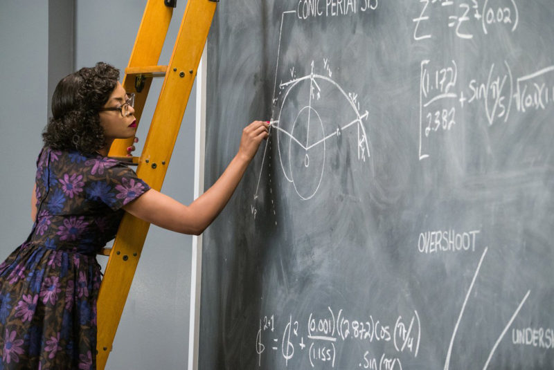
The Euler method is simple, quick to implement, and easy to understand. A true classic when it comes to numerical integration. It even made an appearance in the biographical drama movie Hidden Figures, in which Katherine Johnson used it to calculate the re-entry of austronaut John Glenn from Earth orbit. However, where it gains in simplicity, it loses in accuracy and stability. The \( \mathcal{O}(\Delta t) \) error makes it quite unstable, especially when used in the simulation of soft bodies such as ropes or cloths, where we need to keep track of a lot of particles interacting with each other. What this means in practice is that should we use the Euler method to simulate the rope, it would just go crazy and be all over the place. We don't want that.
1.2.4 Verlet Integration
The Verlet integration method is another integrator often used to solve Newton’s equations of motion numerically. It comes with improved stability, time reversability, and ease of collision handling—all of this at no extra computational cost compared to the Euler method.
In the Euler method we use the approximation with the tanget. How can we improve on that? Well, suppose we know the value of some function g at \( 0 \) and that it’s also infinitely differentiable at \( 0. \) We can say that \[ g(\Delta t) = g(0) + \int_{0}^{\Delta t} g'(t) \, dt. \] Note that since t goes from \( 0 \) to \( \Delta t \) inside the integral, we can replace it with \( \Delta t - t \) without changing the end result: Integrate by parts to get If we keep integrating by parts and then take \( f(t + \Delta t) = g(\Delta t) , \) we obtain what we call the Taylor expansion of f at t: Note that if we only keep terms linear in \( \Delta t, \) we obtain the formula used in the Euler method. We can improve the accuracy by adding more and more higher order terms. However, if we want to approximate the position, we can’t go higher than quadratic, since that would require us to know \( s^{(3)}(t) = a'(t). \) We could choose to go only with terms that are quadratic or lower: and the local error would be \( \mathcal{O}(\Delta t^3). \) Unfortunately, we would not be able to use the same approach for \( v \) because, again, it would require us to know \( a'(t). \) The good news is that we can employ a mathematical trick to get rid of \( v \) and all other odd order derivatives entirely. If we expand \( f(t - \Delta t) \): and then add both expansions together, we get By subtracting \( f(t - \Delta t) \) from both sides and giving up all the terms that are higher than quadratic, we obtain the final approximation formula This is the formula used in Verlet integration. Similarly to the Euler method, the Verlet method says that we can repeatedly apply it to integrate, in our case, the equations of motion. Note that we only need to do it for the position—the velocity is implicit.
To get a better understanding, let’s take a closer look at it. The first thing to note is that there is no first derivative term, we only use the second derivative. If \( f = s, \) the position of some particle, note how the right-hand side can be rewritten as But \( s(t) - s(t - \Delta t) \) divided by \( \Delta t \) is just the average velocity of the particle between times \( t - \Delta t \) and \(t\). In other words, to approximate \( s(t + \Delta t), \) with Euler we had to add the current instantaneous velocity times \( \Delta t \) to \( s(t), \) but with Verlet we have to add the average velocity between the previous interval, from \( t - \Delta t \) to t, times \( \delta t \) and the instantaneous acceleration acceleration times \( \Delta t^2 \).
It turns out that making these two simple changes improves the global error from \( \mathcal{O}(\Delta t) \) to \( \mathcal{O}(\Delta t^2). \) Not perfect, but this together with ease of implementation, the implicit velocity term, and low computational cost, makes Verlet an especially good choice for an integrator in a soft body simulation.
In pseudocode, a procedure using the Verlet integration method to update the positions of a set of particles might look as follows:
| 1 | function simulateVerlet(\(\Delta t\), particles) |
| 2 | for all particles p do |
| 3 | positionCopy \(\leftarrow\) p.position |
| 4 | p.position \(\leftarrow\) \(2 \times \)p.position \(-\) p.previousPosition + \(\Delta t^2 \,\)p.getAcceleration() |
| 5 | p.previousPosition \(\leftarrow\) positionCopy |
Keep in mind that, while we don't need to keep track of the velocity, we do need to keep track of the last two values of the position, instead of just the last one.
Let us compare the Verlet and the Euler methods when it comes to simulating orbits. In the example below, you may press anywhere to create a set of two balls. You may press and drag to choose their initial velocities. The balls are attracted to the large body in the center, with a force that is proportional to the product of their masses, and inversely proportional to the square of the distance between them and the center, as dictated by Newton’s law of universal gravitation. Both are created with identical initial conditions (except for their positions, which are reflections of each other with respect to the center). However, the trajectory of the red ball is determined by the Euler method, while the trajectory of the blue ball is determined by Verlet integration.
Notice how the Verlet balls tend to stay in orbit, while the Euler balls tend to escape. This is because the Euler method is inaccurate at steep changes in velocity, which is exactly the case here as the balls approach the center.
1.2.5 The Jakobsen Method—Enforcing Constraints
To actually build a rope, we create a set of particles that are affected by gravity, and we use Verlet integration to update their positions. To actually look like a rope, these particles need to be constrained to stay close to one another, in a chain of particles.
The constraints may be of the following form: any two particles adjancent in the chain must always be at distance equal to \( d \) from each other, but it also works with inequalities. It depends on what effect we're looking for.
How do we enforce constraints when using Verlet integration? There is one widely known method, which we are going to use. It was first introduced by Thomas Jakobsen in his influencial paper, Advanced Character Physics, written during the development of Hitman: Codename 47 and presented at GDC 2001. We are going to refer to this method as the Jakobsen method.
Say we have two particles at positions v and w, and we would like them to be within distance \(d\) of each other at all times. After running Verlet integration to simulate gravity and other forces, we realize that our particles are now at distance \( d + \Delta d \) of each other, where \( \Delta d = \lVert w - v\rVert - d. \) To enforce the constraint, we just move the particles towards or away from each other such that the constraint becomes satisfied again. Usually, each is moved by a distance \(\left|\Delta d / 2\right|\) units. It may also happen that one particle is fixed and should not be moved, in which case the other one compensates by being moved the entire distance \(\left|\Delta d\right|\). One may also take mass into account and more heavier particles less than lighter ones.
In summary, positions are updated like this: \[ \begin{align} r &\leftarrow \frac{w - v}{\lVert w - v\rVert} \text{ (the unit vector pointing from } v \text{ towards } w \text{)}, \\ v &\leftarrow v + r \frac 1 2 \Delta d \text{ (} v \text{ moves towards } w \text{)}, \\ w &\leftarrow w - r \frac 1 2 \Delta d \text{ (} w \text{ moves towards } v \text{)}. \end{align} \]
We call this operation relaxation, or projection, as the particles are projected on the ends of the inner segment of length d. In pseudocode, we could write
| 1 | function relaxConstraint(particle1, particle2, desiredDistance) |
| 2 | direction \(\leftarrow\) normalize(particle2.position \(-\) particle1.position) |
| 3 | \(\Delta d\) \(\leftarrow\) distance(particle1, particle2) \(-\) desiredDistance |
| 4 | particle1.position.add(\(\Delta d\,\)direction \(/\) 2) |
| 5 | particle2.position.subtract(\(\Delta d\,\)direction \(/\) 2) |
Now, the Jakobsen method is just doing this repeatedly a number of times:
| 1 | function jakobsen(constraints, n) |
| 2 | repeat \(n\) times |
| 3 | for all constraints \( \{ \text{particle1, particle2, desiredDistance} \} \) |
| 4 | \( \text{relaxConstraint}(\text{particle1, particle2, desiredDistance})\) |
Roughly speaking, we define a system as a set of particles and constraints. We call relaxation pass, or projection pass, the operation of relaxing all constraints in the system exactly once. For a system of two particles linked together, one pass is enough to satisfy the constraint entirely. In the case of the rope (a system with more particles linked in a chain) any number of passes won't satisfy all constraints completely. However, the more passes we do, the closer we get to a state where all of them are perfectly satisfied. Theoretically, an infinite number of passes would satisfy all constraints perfectly. The Jakobsen method says that it suffices to do a finite number of passes in order to obtain a believable result. The exact number depends on the number of particles and the constraint model, and remains to be determined empirically.
1.2.6 The Rope
We now have all the mathematical tools to simulate a rope, and it can be done in three simple steps:
- simulate forces on particles using Verlet integration,
- enforce constraints using the Jakobsen method,
- repeat.
The result may be seen below.
Finally—the rope, but why stop here? An entire two-dimensional cloth object can be simulated in the same way—instead of constraining the particles to stay in a line, they are constrained to stay in a grid. Check this box to enable cloth mode in the example above.
So this is how we may implement a simple rope, or even a simple piece of cloth. Let us now take a step back and examine the theory behind in more depth. In what follows, we are going to use slightly more formal mathematics.
1.2.7 A Quick Look at the Jakobsen Method
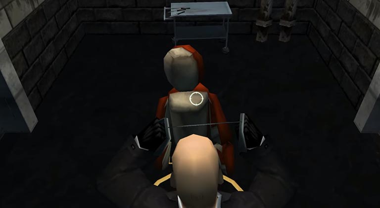
Thomas Jakobsen devised his method as the head of research at IO Interactive, while working on Hitman: Codename 47, a game which I replayed many times.
The game featured realistic ragdolls that the player could interact with. A first glimpse of this new system was present in the tutorial level, where the player was taught how to use a couple of items on an actual ragdoll, setting the expectations for what was to come.
The paper was published in the format of an HTML page, and was presented at Game Developers Conference 2001. It has since been cited many times, becoming somewhat of a de facto resource when diving into the world of soft bodies simulation.
The paper doesn't argue why the method works, formalizations were published later (more about those in the next section). In this section we'll take a closer look at the Jakobsen method in the hopes of obtaining some insights at an intuitive level.
As we saw in the article, the Jakobsen method works by repeatedly “relaxing” the constraints of the system in what we call “passes.” It works directly on positions because of the implicit velocity in Verlet integration. At first, this method of repeatedly relaxing all constraints and hoping for the best may seem naïve, but works well in practice. How does it manage to do so? There is no straightforward answer to this question, but we can get a better understanding by taking a look at a simple example—a system made only of three particles in one a dimensional space. We call them particle \(1\), \(2\), and \(3\), with positions \(x_1\), \(x_2\), and \(x_3\), and contraints: \[ \begin{align} \lvert x_1 - x_2 \rvert &= d, \\ \lvert x_2 - x_3 \rvert &= d \end{align} \] for some chosen distance \(d\). Without loss of generality, suppose the system starts in a state where \[ \begin{align} x_1 &= 0, \\ x_2 &= d + \Delta d_1, \\ x_3 &= x_2 + d + \Delta d_2, \\ \end{align} \] where \( \Delta d_1 \) and \( \Delta d_2 \) are positive numbers. The first step in the first pass relaxes the constraint between \( x_1 \) and \( x_2 \) as such: \[ \begin{align} r &\leftarrow \frac{x_2 - x_1}{\lvert x_2 - x_1 \rvert} \\ x_1 &\leftarrow x_1 + \frac{\Delta d_1}{2} r \\ x_2 &\leftarrow x_2 - \frac{\Delta d_1}{2} r. \end{align} \] When subtracting \( r\, \Delta d_1 / 2 \) from \( x_2 \), the length from \( x_2 \) to \( x_3 \) changes from \( d + \Delta d_2 \) to \( d + \Delta d_1 / 2 + \Delta d_2. \) Below you can find a table with the lengths of the segments between the particles after each pass and relaxation.
| Pass | Operation | \(\lvert x_1 - x_2 \rvert \) | \(\lvert x_2 - x_3 \rvert \) |
|---|---|---|---|
| None | \(d + \Delta d_1 \) | \(d + \Delta d_2 \) | |
| Pass 1 | Relax c. \(1\) | \(d\) | \(d + \Delta d_1 / 2 + \Delta d_2\) |
| Relax c. \(2\) | \(d + \Delta d_1 / 4 + \Delta d_2 / 2\) | \(d\) | |
| Pass 2 | Relax c. \(1\) | \(d\) | \(d + \Delta d_1 / 8 + \Delta d_2 / 4\) |
| Relax c. \(2\) | \(d + \Delta d_1 / 16 + \Delta d_2 / 8\) | \(d\) | |
| \(\vdots\) | |||
| Pass \(n\) | Relax c. \(1\) | \(d\) | \(d + \Delta d_1 / 2^{2n-1} + \Delta d_2 / 2^{2n-2}\) |
| Relax c. \(2\) | \(d + \Delta d_1 / 2^{2n} + \Delta d_2 / 2^{2n-1}\) | \(d\) | |
As it can be seen in the table, after \(n\) passes, the second constraint is always satisfied. Only the first constraint remains unsatisfied, with an error equal to \( \left( \Delta d_1 + 2\Delta d_2 \right) / 2^{2n} \) that goes to \(0\) as \(n\) goes to infinity.
In this particularly small case the algorithm works. Below you can find an animation of how it works when there are 10 particles in a one dimensional system. Segments are represented as red rectangles when their length is far from the target length d. They turn blue as their length gets closer to d. Note that this process, theoretically, doesn't really ever end, but at some point it gets so close to satisfying all constraints completely that you won't be able to notice its progress anymore.
The idea of pass can be observed clearly in this example. You can see how a completely relaxed constraint in complete blue goes from left to right as the algorithm completes the pass. You can see how, with each pass, the system moves closer to satisfying all of its constraints. Error is eliminated from the system at each first and last steps of the pass.
Of course, a trivial example with only one dimension may not do much to help us understand how it works at an intuitive level. Things get more interesting in two-dimensional environments. Let us visualize one more example—this time in 2D.
Unfortunately, no matter how many examples we visualize, they can’t formally prove anything about the algorithm. Of course, one does not need to understand the theoretical backbone of this and other similar methods in order to use them in practice, but for those who want some mathematical insight, let us dive into the field of position based dynamics.
1.2.8 Position Based Dynamics
The classic way of simulating dynamic systems is force based. What this means is that in order to find the positions of some particles in a system, one looks at the forces acting on those particles and infers their positions by means of numerical integration. Because it can offer very high accuracy, this approach is usually used in fields where accuracy is important, such as in computational chemistry or computational physics. In computer games, however, accuracy is not necessary. Believability and simplicity are more desirable features.
In 2006, Matthias Müller, Bruno Heidelberger, Marcus Hennix, and John Ratcliff published a paper titled Position Based Dynamics. They argued that in the case of computer games and other systems that do not require a high degree of accuracy, we may skip the forces and instead work directly on positions. This is exactly what we did with the Jakobsen method when we enforced constraints by directly manipulating the positions of the particles. Jakobsen, along with Müller, actually ended up being considered a founder of the field.
With this approach, we forego some accuracy in exchange for speed and controllability. Both of these are useful in the case of video games, since games need to be both fast and interactive.
Let us define the problem in formal terms. We have a set of \( n \) particles, \( P = \{ 1, 2, \dots, n \} \) and a set of c constraints, \( C = \{ 1, 2, \dots, m \}. \) Although the exact choice of how to define each of these is not set in stone, let us choose to define a particle \( p \in P \) as follows:
- a position \( x_p \in \mathbb{R}^3, \)
- a velocity \( v_p \in \mathbb{R}^3, \)
and define a constraint \( c \in C \) to be made up of
- a function \( f_c : \mathbb{R}^{3n} \rightarrow \mathbb{R} \) that takes in a vector \( [x_1; x_2; \dots; x_n] \) that is a concatenation of the components of the positions of all particles,
- a relation \( \succ_c \) that is either \( = \) or \( \ge \) such that when \( f_c(x) \succ_c 0 \) is true, we say the constraint is satisfied.
At each step we want to simulate the physics of the particles in the system based on their positions and velocities while keeping the constraints satisfied. The first part may be achieved by the use of a numerical integrator, such as Euler or Verlet. The problem is that this simulation substep may break the constraints. Thus, before the final result is returned, we need to add in another substep in which the positions are adjusted such as to keep the constraints satisfied. Usually, in practice, we won't be able to satisfy all of them perfectly, so we resort to an approximation.
Mathematically, to fix the constraints, we need to solve (i.e. find an approximate solution to) the system of non-linear equations \[ f_c(x) \succ_c 0, \forall c \in C. \]
Even though the system we are dealing with is non-linear, let us for a moment take a step back and present a set of methods that deal with system of linear equations. Then we are going to see how we can generalize them for non-linear systems.
Iterative Methods for Solving Linear Systems
Suppose we have a square linear system of equations \( Ax = b. \) Suppose, however, that the matrix A is too complicated to work with directly. What we can do instead is replace it with a new matrix M and move the difference \( A - M \) to the other side of the equation: \[ Mx = (A - M)x + b. \] Now, if we need an exact solution, we are still forced to deal with A, nothing changes. On the other hand, if an approximation suffices, we may solve this new equation iteratively as follows. We begin with an initial guess \( x^{(0)} \) and at each step we take the current \( x^{(k)} \) and find an even better approximation \( x^{(k + 1)} \) by solving \[ Mx^{(k)} = (A - M)x^{(k + 1)} + b. \] This equation may be simpler, but it never gives the exact solution—we need to keep solving it over and over. In practice, we keep solving it until the error is below some desired threshold, or as long as the time budget allows.
On top of that, not every M will work. Intuitively, the closer it is to A, the faster the iteration converges to the exact solution. \( M = A \) converges in just one interation. On the other hand, M also needs to be as simple as possible. There are, in fact, three choices of M that are both simple and with good convergence rates when they do converge:
- \( M_1 = \text{the diagonal part of } A \) (the Jacobi method),
- \( M_2 = \text{a triangular part of } A \) (the Gauss-Seidel method),
- \( M_1 + M_2 \) (successive overrelaxation).
Keep in mind that the convergence of \( x^{(k)} \) when \( k \rightarrow \infty \) is not guaranteed. However, if \( x^{(k)} \) does converge to some \( x^{(\infty)} \) as \( k \rightarrow \infty, \) it is true that \( A x^{(\infty)} = b, \) i.e. \( x^{(\infty)}, \) if it exists, is the correct solution to our initial system of equations.
Let us direct our attention to the choices \( M_1 \) and \( M_2 \) for the matrix M, and how the Jacobi and the Gauss-Seidel methods act on individual components of \( x^{(k)}. \) In the case of Jacobi, we have \[ x_i^{(k + 1)} = \frac{1}{a_{ii}} \left( b_i - \sum_{j \neq i } a_{ij} x_j^{(k)} \right). \] Note here that to find \( x_i^{(k + 1)}, \) Jacobi only uses the components of \( x^{(k)}. \) Thus, the components of \( x^{(k + 1)} \) can be computed independently and in parallel. On the other hand, with Gauss-Seidel we have Let us take a moment and understand how this formula is different from Jacobi’s. They are quite similar, but there is one key difference. With Gauss-Seidel, after a component \( x_i^{(k + 1)} \) is computed, it is then used in the computation of all subsequent components \( x_j^{(k + 1)}, j > i. \) We make use of new approximations as they become available. This is similar to what we did with the Jakobsen method.
As you might have noticed, all of these methods are for linear systems, but we are dealing with a non-linear system. The good news is that we can employ a mathematical trick to overcome this impediment.
Non-Linear Gauss-Seidel
We are going to focus our attention on the Gauss-Seidel method, but the technique we are going to use to liniarize the non-linear system is compatible with the other two iterative methods as well.
As a reminder, the system we are trying to solve is \[ f_c(x) \succ_c 0, \forall c \in C, \] where x represents the concatenation of the position vectors of the particles in the system. Instead of solving the entire system at once, we are going to solve each equation \( f_c(x) \succ_c 0, \) for a specific c, individually. In similar Gauss-Seidel fashion, after we find a solution x given by the condition of some constraint c, we use it as a starting point to find a solution to the equation given by the next constraint. In this way, we keep finding values for x that, as we'll see, converge to a state where all the constraints are perfectly satisfied.
After x is updated to satisfy the condition of some constraint c, we say that the constraints c is relaxed. With this in mind, we say that our algorithm works by successively relaxing all the constraints in the system.
But how do we relax a constraint? Each one yields one scalar equation \( f_c(x) \succ_c 0 \) with up to \( 3n \) unknowns. This is an underdetermined non-linear system. Let us frame the problem as follows: given an initial value for \( x, \) say \( x^{(k)}, \) we want to find a correction \( \Delta x \) such that \( f_c(x^{(k)} + \Delta x) \succ_c 0 . \) Then we say \( x^{(k + 1)} \) is \( x^{(k)} + \Delta x. \) Now we need to find \( \Delta x \) instead, but it’s still a non-linear system. Fortunately we may employ the concept of linearization around a point, in this case \( x^{(k)} \): where \( \nabla f_c(x^{(k)}) \) is the gradient of \( f_c \) at \( x^{(k)}, \) a vector made up of all the partial derivatives with respect to each component of \( x^{(k)}. \) The system is now linear, but still underdetermined. This is mended by restricting \( \Delta x \) to be in the direction of \( \nabla f_c(x^{(k)}). \) The problem is now reduced to finding one scalar \( \lambda \) such that \[ f_c(x^{(k)}) + \lambda \lVert \nabla f_c(x^{(k)}) \rVert^2 \succ_c 0. \] This results in \[ \lambda = -\frac{f_c(x^{(k)})}{ \lVert \nabla f_c(x^{(k)}) \rVert^2 } \] and thus \[ \Delta x = -\frac{f_c(x^{(k)})}{ \lVert \nabla f_c(x^{(k)}) \rVert^2 } \nabla f_c(x^{(k)}). \] To get a better understanding, let us zoom in and inspect what happens in the case of just one particle \( p \in P. \) First, note that the numerator, which is the squared length of the gradient, can be rewritten as the sum of the squared lengths of the subvectors of the gradient: \[ \lVert \nabla f_c(x^{(k)}) \rVert^2 = \sum_{p \in P} \Big\lVert \left[ \nabla f_c(x^{(k)}) \right]_p \Big\rVert^2, \] where \( \left[ \nabla f_c(x^{(k)}) \right]_p \) is the subvector of the gradient that contains only the partial derivatives with respect to components of \( x_p. \) Consequently, the correction for a single particle p is This formula is something we could use in practice. In fact, we did use it when we implemented the Jakobsen method. Let us again consider the case of two particles and a single constraint with the function \[ f(x = [ x_1; x_2 ]) = \lVert x_1 - x_2 \rVert - d \] which is satisfied when \( f(x) = 0. \) We have that \[ \nabla f(x) = \frac{[ x_1 - x_2; x_2 - x_1 ]}{\lVert x_1 - x_2\rVert} \] and thus \[ \begin{align} \big[ \nabla f(x) \big]_1 &= \frac{x_1 - x_2}{\lVert x_1 - x_2\rVert}, \\ \big[ \nabla f(x) \big]_2 &= \frac{x_2 - x_1}{\lVert x_1 - x_2\rVert}. \end{align} \] For \( \lambda \) we have \[ \lambda = - \frac{ \lVert x_1 - x_2 \rVert - d }{ 2 }. \] Let us say that \( \Delta d = \lVert x_1 - x_2 \rVert - d. \) Finally, we get the individual corrections: \[ \begin{align} \Delta x_1 &= \frac{ \Delta d (x_2 - x_1) }{ 2 \lVert x_1 - x_2 \rVert }, \\ \Delta x_2 &= \frac{ \Delta d (x_1 - x_2) }{ 2 \lVert x_1 - x_2 \rVert }, \end{align} \] which are the exact same corrections we used in our implementation of the Jakobsen method.
Masses, Stiffness, and More
There are many more features we could add to our simulation. Masses may be incorporated by using the inverse of a \(3n\) by \(3n\) mass matrix \[ M = \begin{bmatrix} m_1 & 0 & 0 & 0 & \dots & 0 \\ 0 & m_1 & 0 & 0 & \dots & 0 \\ 0 & 0 & m_1 & 0 & \dots & 0 \\ 0 & 0 & 0 & m_2 & \dots & 0 \\ \vdots & \vdots & \vdots & \vdots & \ddots & 0 \\ 0 & 0 & 0 & 0 & \dots & m_n \end{bmatrix} \] (where \( m_p \) is the mass of the particle p) to transform the gradient in the computation of \( \Delta x \) as such \[ \Delta x = \lambda M^{-1} \nabla f_c(x^{(k)}). \] Stiffness may be introduced in various ways. For example we may multiply the correction by a stiffness constant \( k \in [0 \dots 1] \) when applying the correction as such: \[ x^{(k + 1)} \leftarrow x^{(k)} + k \Delta x. \] This is, unfortunately, dependent on the number of iterations we do, but can be fixed by doing \[ x^{(k + 1)} \leftarrow x^{(k)} + \big(1 - \left(1 - k\right)^s\big) \Delta x, \] instead, where \( s \) is the number of iterations.
1.3 Conclusion
We saw how to implement a basic rope simulation. We also briefly examined the mathematical framework that sits behind the implementation we used. Let me end this by highlighting that there are many more features one could add to this implementation. Of course, there are also other ways, including completely different mathematical frameworks, to achieve the same effect. For example, instead of position based dynamics, one might use a spring-mass model—this would be more like the “traditional” way of doing a physics simulation, one where we don't skip the force and velocity layers when enforcing constraints.
A word of warning, though—soft bodies are ferocious creatures. They can quickly devour the CPU and / or GPU if used excessively. Using them in complex three-dimensional worlds where many other things need to be going on at the time needs to be done with care. They may drive down performance significantly, especially on older and less powerful machines.
On the other hand, they can provide that extra something to your game, that extra kick that can make the difference between a dull and an immersive environment. They can make the world you're building seem more lively by bringing a touch of softness in a sea of rigid objects.
1.4 See Also
I hope all of this seemed interesting to you. If all of this was new, I admit, it’s not the easiest of subjects to get into, so I thank you for making the effort. If you want to dive deeper, let me point you towards some resources that might aid you in your journey.
-
 Foundations of Physically Based Modeling and Animation
by Donald House and John C. Keyser, published by CRC Press in 2016. See sections 7.2.2 about Velocity Verlet, a method that is mathematically equivalent to standard Verlet, but explicitly computes the velocity, in case you need it in your calculations. Also, see section 7.2.3 about leapfrog integration—one other way to integrate the laws of motion.
Foundations of Physically Based Modeling and Animation
by Donald House and John C. Keyser, published by CRC Press in 2016. See sections 7.2.2 about Velocity Verlet, a method that is mathematically equivalent to standard Verlet, but explicitly computes the velocity, in case you need it in your calculations. Also, see section 7.2.3 about leapfrog integration—one other way to integrate the laws of motion.
-
 Numerical Recipes: The Art of Scientific Computing (Third Edition)
by William H. Press, Saul A. Teukolsky, William T. Vetterling, and Brian P. Flannery, published by Cambridge University Press in 2007. A bit heavier with the math, this book is a fabulous treatment of all kinds of numerical methods. I recommend chapter 2 (solving systems of linear equations), chapter 17 (integrating ordinary differential equations), and chapter 20 (solving partial differential equations). A brief overview of the Gauss–Seidel and Jacobi methods can also be found at the beginning of section 20.5.
Numerical Recipes: The Art of Scientific Computing (Third Edition)
by William H. Press, Saul A. Teukolsky, William T. Vetterling, and Brian P. Flannery, published by Cambridge University Press in 2007. A bit heavier with the math, this book is a fabulous treatment of all kinds of numerical methods. I recommend chapter 2 (solving systems of linear equations), chapter 17 (integrating ordinary differential equations), and chapter 20 (solving partial differential equations). A brief overview of the Gauss–Seidel and Jacobi methods can also be found at the beginning of section 20.5.
-
 Introduction to Applied Mathematics
by Gilbert Strang, published by Wellesley Cambridge Press in 1986. This comes as a more general recommendation. The way I explained the Jacobi and Gauss-Seidel methods is highly inspired by this book (section 5.3—Semi-Direct and Iterative Methods), so make sure to check it out. The entire book is a must-read for anyone who is serious about getting into applied mathematics. I might be biased here, but I think everything that has written the name Gilbert Strang on the cover is worth a read. He simply is one of the best teachers and writers I know.
Introduction to Applied Mathematics
by Gilbert Strang, published by Wellesley Cambridge Press in 1986. This comes as a more general recommendation. The way I explained the Jacobi and Gauss-Seidel methods is highly inspired by this book (section 5.3—Semi-Direct and Iterative Methods), so make sure to check it out. The entire book is a must-read for anyone who is serious about getting into applied mathematics. I might be biased here, but I think everything that has written the name Gilbert Strang on the cover is worth a read. He simply is one of the best teachers and writers I know.
-
Really anything that Matthias Müller and Miles Macklin publish out of the research division at NVIDIA. Below you can find a list of some specific publications that my be a good next step in studying position based dynamics.
- Position Based Dynamics—the original 2006 position based dynamics paper.
- Position Based Fluids—using the position based dynamics framework for simulating fluids.
- Position Based Simulation Methods in Computer Graphics 2017—not a research paper, but the course notes from an EUROGRAPHICS 2017 tutorial—a very good overview of the field which I used extensively in the writing this article.